CLP(FD) and CLP(ℤ): Prolog Integer Arithmetic
It is rather as if the professional community had been suddenly
transported to another planet where familiar objects are seen in
a different light and are joined by unfamiliar ones
as well. (Thomas S. Kuhn, The Structure of
Scientific Revolutions)
Introduction
To fully appreciate declarative integer arithmetic
in Prolog, let us first consider arithmetic
over natural numbers as a simpler special case.
The natural numbers are defined by
the Peano axioms.
In particular, 0 is a natural number, and for every
natural number n,
its successor S(n) is also a
natural number. Thus, we could use the following
Prolog program to define the set of natural numbers:
natnum(0).
natnum(s(N)) :-
        natnum(N).
In this representation, the natural number 0 is represented
by the Prolog integer 0, and
the successor of any natural number N is
represented by the
compound term s(N). For
example, the integer 2 is represented as s(s(0)),
since it is the successor of the successor of zero. This
representation is variously
called successor arithmetic, successor notation
and also Peano arithmetic.
With this representation, we could use the following
Prolog program to define addition, which is
a relation between two natural numbers and
their sum:
Exercise: Suppose I replace the goal nat_nat_sum(M,
N, Sum) by nat_nat_sum(N, M, Sum). What are the
advantages, and what are the drawbacks of this change, if any?
nat_nat_sum(0, M, M).
nat_nat_sum(s(N), M, s(Sum)) :-
        nat_nat_sum(M, N, Sum).
This is a pure predicate
that terminates if any of the arguments is instantiated. We
can read the
clauses declaratively to reason
about the cases that this relation describes. Other elementary
relations between natural numbers can be defined analogously.
Unfortunately, this representation of natural numbers suffers
from several significant disadvantages:
- First, this is not really the way we want to write
and read numbers. We would like to use a more familiar
notation—such as 1, 2 and 3—to represent
natural numbers.
- With some practice, we may get used to the
successor notation. However, a more fundamental problem
remains: This representation takes space that is directly
proportional to the magnitude of the numbers we
need to represent. Thus, the space requirement
grows exponentially with the length of any number's
decimal representation. Therefore, reasoning about larger
numbers is infeasible with this representation.
- More complex relations such as multiplication
and exponentiation are hard to define in such a way
that they work in all directions and retain good
termination properties.
- To extend this representation to integers, we also
need a way to represent negative numbers.
Therefore, successor notation—albeit useful to illustrate
different ways in which we could represent
our data—is not how we typically reason
about numbers in Prolog.
Instead, we use
built-in predicates to reason
about numbers in Prolog. In the case of integers,
these predicates are known as CLP(FD) constraints, and
in more recent systems also
as CLP(ℤ) constraints. CLP(FD) stands
for Constraint Logic Programming
over Finite Domains and reminds us of the fact that in
reality, we can only represent a finite subset of integers
on actual machines. ℤ denotes the integers
and indicates that these constraints are designed for reasoning
about all integers.
All widely used Prolog implementations provide
CLP(FD) constraints. However, the exact details differ
slightly between various systems. For example, in GNU Prolog,
B-Prolog and other systems, CLP(FD) constraints are conveniently
available right from the start. In contrast, you need to load
a library to use them in SICStus Prolog and
other systems.
If your Prolog systems provides these constraints as a library,
adjust your initialization file so that this library is
automatically available in all your programs. For example, in
Scryer Prolog, you can put the following directive in your
~/.scryerrc initialization file:
:- use_module(library(clpz)).
It is highly advisable to make CLP(FD) or CLP(ℤ) constraints
automatically available in all your programs, since almost all
Prolog programs also reason about integers.
| Video: |
|
Constraints
Generally, an n-ary constraint is a relation
between n variables. For example, (=)/2
and dif/2 fit this definition: These predicates
are also constraints! In fact, every predicate you
impose can be regarded as a constraint on the set
of solutions.
In the following, we are considering CLP(FD) constraints.
These are built-in predicates that enable reasoning
over integers in a pure and declarative way.
The most important CLP(FD) constraints are the arithmetic
constraints (#=)/2, (#<)/2, (#>)/2
and (#\=)/2:
| Constraint |
Meaning |
|
A #= B
|
A is equal to B
|
A #< B
|
A is less than B
|
A #> B
|
A is greater than B
|
A #\= B
|
A is not equal to B
|
In this table, A and B are
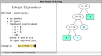
arithmetic expressions. Expressions are
defined inductively:
- a variable is an expression
- an integer is an expression
- if X and Y are
expressions, then X+Y, X-Y
and X*Y are also expressions.
There are several more cases of arithmetic expressions, and also
other categories of constraints, such as combinatorial
constraints. See your Prolog system's manual for more
information.
Evaluating integer expressions
The most basic use of CLP(FD) constraints is evaluation of
arithmetic expressions.
To evaluate integer expressions, we use the
predicate (#=)/2 to denote equality of arithmetic
expressions over integers.
Here are a few examples:
?- X #= 5 + 3.
   X = 8.

?- 2 #= X + 9.
   X = -7.

?- 1 #= 1 + Y.
   Y = 0.
Equality is one of the most important predicates when reasoning
about integers. As these examples illustrate, (#=)/2 is a
pure relation that can be used in all
directions, also if components of its arguments are still variables.
Example: Length of a list
For example, we can readily relate
a list to its length as follows:
list_length([], 0).
list_length([_|Ls], Length) :-
        Length #= Length0 + 1,
        list_length(Ls, Length0).
A declarative reading of this
predicate makes clear what this relation means:
- The length of the empty list is 0.
- If Length0 is the length
of Ls and Length
is Length0 plus 1, then the length
of [_|Ls] is Length.
Example query:
?- list_length("abcd", Length).
   Length = 4.
Importantly, this also works in more general cases. For example:
?- list_length(Ls, Length).
   Ls = [], Length = 0
;  Ls = [_A], Length = 1
;  Ls = [_A,_B], Length = 2
;  Ls = [_A,_B,_C], Length = 3
;  ... .
It can also be used in a different direction. For example:
?- list_length(Ls, 3).
   Ls = [_A,_B,_C]
;  ... .
Note though that this does not terminate:
?- list_length(Ls, 3), false.
nontermination
It takes only a single additional goal to make this
query terminate. This is left as an exercise.
To avoid the accumulation of constraints, we can introduce
an explicit accumulator. By this, we mean a term that
represents intermediate states that arise. For example, here is
an alternative solution for relating a list to
its length:
list_length(Ls, L) :-
        list_length_(Ls, 0, L).

list_length_([], L, L).
list_length_([_|Ls], L0, L) :-
        L1 #= L0 + 1,
        list_length_(Ls, L1, L).
Again, making the goal list_length(Ls, 3) terminate is left as an exercise.
Domains
We can reason even more generally over integers. Consider a
variable V that we want to use as a
placeholder for an integer between 0 and 2. We express this
on the toplevel using the constraint (in)/2:
?- V in 0..2.
   clpz:(V in 0..2).
If we place additional goals on the toplevel, the system
automatically takes into account the admissible set of integers we
specified for V, which we call its associated
domain. In particular, the system prevents us from unifying
V with integers that are not elements of its domain:
?- V in 0..2, V #= 3.
   false.
In contrast, the following query succeeds:
?- V in 0..2, V #= 1.
   V = 1.
Now two variables X and Y, both constrained to
the interval 0..2:
?- X in 0..2, Y in 0..2.
   clpz:(X in 0..2), clpz:(Y in 0..2).
Or, equivalently:
?- [X,Y] ins 0..2.
   clpz:(X in 0..2), clpz:(Y in 0..2).
Thus, the predicate (ins)/2 lifts (in)/2
to lists of variables.
Labeling
We can successively bind a variable to all integers of its
associated domain via backtracking, using the enumeration
predicate indomain/1:
?- V in 0..2, indomain(V).
   V = 0
;  V = 1
;  V = 2.
Assigning concrete values to constrained variables is called
labeling. The predicate label/1
lifts indomain/1 to lists of variables:
?- [X,Y] ins 0..1, label([X,Y]).
   X = 0, Y = 0
;  X = 0, Y = 1
;  X = 1, Y = 0
;  X = 1, Y = 1.
If label/1 were not available, you could define it like this:
label(Vs) :- maplist(indomain, Vs).
Labeling is a form of search
that always terminates. This property is of extreme
importance for termination analysis and allows us to cleanly
separate the modeling part from the actual search.
In practice, the order in which variables are bound to concrete
values of their domains matters. For this reason, the
predicate labeling/2, which is a generalization
of label/1, lets you specify different strategies
when enumerating admissible values. A simple and often very
effective heuristics is to always label that variable next whose
domain contains the smallest number of elements. This
strategy is called "first-fail", since these variables are often
most likely to cause failure of the labeling process, and trying
them early can prune huge portions of the search tree. It is
available via labeling([ff], Vars).
For other problems, a static reordering of variables may suffice.
With N-queens for example, it is worth
trying to order the variables so that labeling starts from the
board's center and gradually moves to the borders.
Constraint propagation
From what we have seen above, it follows that we
can combine different constraints by stating them as
a conjunction. For instance, we can state
that Z is the sum of X and Y, both
of which are integers between 0 and 2:
?- [X,Y] ins 0..2, Z #= X + Y.
   clpz:(X+Y#=Z), clpz:(X in 0..2), clpz:(Y in 0..2), clpz:(Z in 0..4).
Note that the domain of Z is deduced from the
posted constraints without being stated explicitly. Narrowing
domains based on posted constraints is called
(constraint) propagation, and it is performed automatically
by the constraint solver. If we bind
Z to 0, the system deduces that both X
and Y are also 0:
?- [X,Y] ins 0..2, Z #= X + Y, Z #= 0.
   X = 0, Y = 0, Z = 0.
In this case, propagation yields ground instances for all
variables. In other cases, constraint propagation detects
unsatisfiability of a set of constraints without any labeling:
?- X in 0..1, X #> 2.
   false.
In yet other cases, domain boundaries are adjusted:
?- [X,Y] ins 0..2, Z #= X + Y, Z #= 1.
   Z = 1, clpz:(X+Y#=1), clpz:(Y in 0..1), clpz:(X in 0..1).
A set of constraints and variables with associated domains is
called (globally) consistent if all variables can be
simultaneously bound to (at least) one value of their respective
domains such that all constraints are satisfied. In general, all
variables must be labeled to find out whether a set of
constraints is consistent. However, there exist weaker forms of
consistency that are guaranteed without labeling.
For example, the all_different/1 constraint does not
detect unsatisfiability of the following:
?- [X,Y,Z] ins 0..1, all_different([X,Y,Z]).
   clpz:all_different([X,Y,Z]), clpz:(X in 0..1), clpz:(Y in 0..1), clpz:(Z in 0..1).
The all_distinct/1 constraint, in contrast, detects the
inconsistency without labeling any variables:
?- [X,Y,Z] ins 0..1, all_distinct([X,Y,Z]).
   false.
To guarantee that stronger form of consistency, the
all_distinct/1 constraint must do extra work for
propagation. It therefore depends on the problem at hand whether
it pays off to use it instead of all_different/1. If
there are many solutions distributed throughout the whole
search space, a naive search for solutions may easily find
them, and additional pruning may only make this process
slower. On the other hand, if solutions are relatively sparse, the
additional pruning of all_distinct/1 can help to
more effectively prune irrelevant parts of the search space.
In practice, all_distinct/1 is
typically fast enough and is preferable due to its
much stronger propagation.
We can generalize this observation: There is a trade-off
between strength and efficiency of constraint
propagation. And further, when reasoning about integers, there
are inherent limits to the strength of constraint
propagation: It follows from
Matiyasevich's theorem
that constraint solving over integers is not decidable
in general. This means that there is no computational method that
always terminates and always correctly decides whether a set
of integer equations has a solution. Therefore, in
general, search—for example
via labeling—must be used to find
concrete solutions, or to detect that none exists.
Legacy predicates
CLP(FD) constraints have been available only for a
few decades. This means that they are still
a comparatively recent development in Prolog systems. Most
available textbooks have not yet had a chance to take such
innovations into account. Many Prolog instructors have
completed their formal education before constraints have become
widely available. As a result, many Prolog programmers have never
even heard of constraints.
Instead of arithmetic constraints like (#=)/2
and (#>)/2, you can also use lower-level
arithmetic predicates like (is)/2
and (>)/2 to reason about integers. However, this
comes with several hefty drawbacks. For example:
- (is)/2 and other low-level predicates
are moded. This means that they can only be used in a
few directions, making them unsuitable for more
general relations. This severe limitation also
prevents declarative debugging.
- (is)/2 and other low-level predicates intermingle
reasoning about integers with reasoning about floating point
numbers, and in some systems even
about rational numbers. This means that when readers
of your code see such predicates, they will wonder whether you
are using them because floating point numbers may
arise somewhere. In contrast, (#=)/2 and other CLP(FD)
constraints make it perfectly clear that you intend to reason
about integers. These constraints will help you to
find certain classes of mistakes in your code more easily,
because they throw type errors instead of failing
silently.
- (is)/2 and other low-level predicates force
beginners to understand the procedural execution of
Prolog programs in addition to understanding the
declarative semantics. This is too hard in almost
all cases.
- (is)/2 itself is not sufficient: You also
need (=:=)/2. In contrast, the CLP(FD)
constraint (#=)/2
subsumes both (is)/2 and (=:=)/2
when reasoning over integers, making Prolog easier to teach.
For these reasons, I regard (is)/2, (>)/2 and
other low-level predicates as legacy predicates. I
expect them to gradually disappear from application code
when the current generation of Prolog instructors is replaced, and
more general techniques are taught instead.
By the way: (=<)/2 is not written
as (<=)/2, because the latter would look too much like
an arrow which is often used
for theorem proving
in Prolog.
Further reading
CLP(FD) constraints let you solve a large variety
of combinatorial
optimization tasks
and puzzles.
Correctness Considerations in CLP(FD)
Systems contains an introduction to CLP(FD) and many
pointers to further literature.
Several CLP(FD) examples are available
from: https://github.com/triska/clpz
More about Prolog
Main page