Combinatorial Optimization with Prolog

Prolog is eminently suitable for solving combinatorial and optimization tasks, such as:

timetabling
resource allocation
planning, i.e., finding suitable orderings of dependent tasks
scheduling
etc.

It is easy to generate and test solutions for such tasks in Prolog. If this is done naively (either in Prolog or with any other language), then it quickly leads to infeasible programs, because there are typically too many combinations to generate them all.

To efficiently solve combinatorial optimization tasks in many cases of practical relevance, Prolog provides a declarative solution called constraints. Importantly, constraints can prune large parts of the search tree before the search even begins, and also while the search is progressing. In typical cases, this is vastly more efficient than naively enumerating solutions. In addition, constraints retain the generality we expect from relations, and so you can use constraint-based Prolog programs for generating, testing and completing solutions of combinatorial tasks.

In principle, constraints can be provided by any programming language. However, they blend in especially seamlessly into logic programming languages like Prolog due to their relational nature and built-in search and backtracking mechanisms. For this reason, logic programming languages have become the most important host languages for constraints, and all widely used Prolog systems ship with several libraries or built-in predicates for constraint solving.

CLP(X) stands for constraint logic programming over the domain X. Plain Prolog can be regarded as a CLP(H): Constraint logic programming over Herbrand terms, with (=)/2 and dif/2 as the most important constraints that denote, respectively, equality and disequality of terms. There are dedicated libraries for several important domains. Support of these libraries differs between Prolog systems, so check your Prolog system's manual for more information.

For example, SICStus Prolog ships with:

CLP(FD) for integers
CLP(B) for Boolean variables
CLP(Q) for rational numbers
CLP(R) for floating point numbers

In Prolog, declarative integer arithmetic can thus be naturally used for solving combinatorial tasks.

Here is an example:

A chicken farmer also has some cows for a total of 30 animals, and the animals have 74 legs in all.

How many chickens does the farmer have?

Answer:

?- Chickens + Cows #= 30,
   Chickens*2 + Cows*4 #= 74,
   Chickens in 0..sup,
   Cows in 0..sup.
Chickens = 23,
Cows = 7.

Note that no search was necessary at all. The constraint solver has deduced the unique solution of the puzzle via constraint propagation.

In industrial and academic use, the efficiency of a Prolog system's constraint solvers is often an important factor when choosing a system. This is because many commercial use cases of Prolog also involve combinatorial optimization tasks.

Integers are the most relevant domain in practice, because all finite domains can be mapped to finite subsets of integers. Hence, all finite combinatorial optimization tasks can be expressed via CLP(FD) constraints.

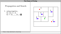
Example: Map Colouring

Let us consider map colouring, i.e., the task of assigning colours to regions of a map in such a way that no adjacent regions are assigned the same colour.

Video:

We can easily map this task to a combinatorial task over integers, by using one variable for each region, and one integer for each colour.

For concreteness, let us colour the following map:

We shall use the integers 0, 1, 2, ..., to represent suitable colours. Moreover, we know from the Four Colour Theorem that at most 4 colours suffice.

The following Prolog program describes the task using CLP(FD) constraints:

regions(Rs) :-
        Rs = [A,B,C,D,E,F],
        Rs ins 0..3,
        A #\= B, A #\= C, A #\= D, A #\= F,
        B #\= C, B #\= D,
        C #\= D, C #\= E,
        D #\= E, D #\= F,
        E #\= F.

Disequality constraints ((#\=)/2) are used to state that pairs of integers that correspond to adjacent regions must be different. To obtain concrete solutions, we use labeling:

?- regions(Rs), label(Rs).
   Rs = [0,1,2,3,0,1]
;  Rs = [0,1,2,3,0,2]
;  Rs = [0,1,2,3,1,2]
;  Rs = [0,1,3,2,0,1]
;  ... .

To obtain more readable solutions, we can relate integers to colours. For example:

integer_color(0, red).
integer_color(1, green).
integer_color(2, blue).
integer_color(3, yellow).

This allows us to query:

?- regions(Rs), label(Rs),
   maplist(integer_color, Rs, Cs),
   pairs_keys_values(Pairs, [a,b,c,d,e,f], Cs).
Rs = [0, 1, 2, 3, 0, 1],
Cs = [red, green, blue, yellow, red, green],
Pairs = [a-red, b-green, c-blue, d-yellow, e-red, f-green] ;
Rs = [0, 1, 2, 3, 0, 2],
Cs = [red, green, blue, yellow, red, blue],
Pairs = [a-red, b-green, c-blue, d-yellow, e-red, f-blue] ;
etc.

These solutions look like this:

The following query shows that at least 4 colours are needed in this case:

?- regions(Rs), Rs ins 0..2, label(Rs).
   false.

Major advantages of using CLP(FD) constraints for combinatorial tasks include:

compactness and elegance of declarative descriptions
efficiency due to powerful pruning
intelligent labeling strategies guided by remaining domains
availability of global constraints tailored for specific applications.

Graphs

Graphs are an extremely important concept in mathematics and computer science, and many combinatorial tasks can be formulated as problems involving graphs. For example, the preceding map colouring task is an instance of a more general task called graph colouring.

We distinguish between directed and undirected graphs.

Directed graphs

A directed graph consists of:

a set V of vertices
a set A of arcs, which are directed edges of the form v→w (v, w ∈ V).

In Prolog, there are different ways to represent directed graphs. One way to do it is to write down the arcs as Prolog facts:

arc_from_to(a, b).
arc_from_to(b, c).
arc_from_to(a, c).
arc_from_to(c, a).

Such a representation is called temporal, because solutions are iteratively reported on backtracking. This representation is very well suited for making large amounts of data efficiently accessible. An example use case is a set of public transport routes between different locations.

A typical way to describe paths with such a representation is:

path_from_to(A, A, _) --> [A].
path_from_to(A, B, Visited) --> [A],
        { arc_from_to(A, Next),
          maplist(dif(Next), Visited) },
        path_from_to(Next, B, [A|Visited]).

We keep track of vertices that have already been visited and ensure that any vertex is visited at most once.

Example queries:

?- phrase(path_from_to(a, c, []), Ps).
   Ps = "abc"
;  Ps = "ac"
;  false.

?- phrase(path_from_to(a, To, []), Ps).
   To = a, Ps = "a"
;  To = b, Ps = "ab"
;  ... .

Using all solutions predicates, we can convert any temporal representation to a spatial representation, i.e., Prolog data structures such as lists:

?- findall(From-To, arc_from_to(From, To), Arcs).
    Arcs = [a-b,b-c,a-c,c-a].

Another example:

?- bagof(To, arc_from_to(From, To), Arcs).
   From = a, Arcs = "bc"
;  From = b, Arcs = "c"
;  From = c, Arcs = "a".

With these predicates, we can obtain a representation of the graph in the form of an adjacency list, where we store which vertices are reachable from any given vertex:

?- findall(From-Ls, bagof(To, arc_from_to(From, To), Ls), Is).
   Is = [a-"bc",b-"c",c-"a"].

In Prolog, this is often a good representation for graphs. We can easily turn this into an association list of the form V→Vs to obtain logarithmic worst case (and expected) access time when fetching the vertices Vs that are reachable from any given vertex V. For utmost efficiency, if your Prolog system supports it, you can represent each vertex as a Prolog variable, and attach information (including arcs) in the form of variable attributes. This even allows destructive modifications in O(1). With this method, you can for example efficiently compute the strongly connected components of a directed graph. See scc.pl for more information.

Note that isolated vertices do not participate in any arc, and so—at least in general—we also need to represent the vertices separately:

vertices([a,b,c,d]).

In the adjacency list representation, the isolated vertex d can be represented as d-[].

Undirected graphs

An undirected graph consists of:

a set N of nodes
a set E of undirected edges of the form x−y (x, y ∈ N).

For example, let us reconsider the map colouring task from a graph theoretic perspective. The CLP(FD) formulation can be regarded as implicitly describing a graph that is induced by the constraints that are stated between the variables. We now make that graph available explicitly as a Prolog term that represents an undirected graph:

edges([a-b,a-c,a-d,a-f,
       b-c,b-d,
       c-d,c-e,
       d-e,d-f,
       e-f]).

edge(X, Y) :- edges(Es), ( member(X-Y, Es) ; member(Y-X, Es) ).

Now we can query:

?- bagof(E, edge(N, E), Es).
   Es = "bcdf", N = a
;  Es = "cda", N = b
;  Es = "deab", N = c
;  Es = "efabc", N = d
;  Es = "fcd", N = e
;  Es = "ade", N = f.

An explicit representation is well suited for further analysis of the graph.

Trees

In graph theory, a tree is an undirected graph in which any two nodes are connected by exactly one path.

In Prolog, trees are of special significance because Prolog terms naturally correspond to trees.

For example, we can fairly enumerate binary trees as follows:

tree(nil) --> [].
tree(node(_, Left, Right)) --> [_], tree(Left), tree(Right).

Sample query: